
Andrew Jesaitis


Accurate variant classification is critical to any clinical variant analysis pipeline. Due to the sheer number of variants that must be processed, we need an automated way of predicting the biological significance of a variant. There are various ways of approaching this problem, but one of the most common is “Model-free Variant Effect Prediction”. Model-free refers to the fact that the method requires no pre-analysis (training) of the algorithm on a separate dataset and effect prediction simply means inferring the biological change rather than producing a quantitative measure of deleteriousness.
In 2014, I looked at the most widely used algorithms that did variant effect prediction – Annovar, SnpEff, and VEP – and found only a moderate degree of concordance. My findings agreed with Davis McCarthy’s analysis which demonstrated that VEP and Annovar only agreed 65% of the time when annotating Loss of Function variants. McCarthy further demonstrated that the choice of transcript set had a similarly large effect when using the same algorithm.
Fast-forward three years to the present day. Is the situation any better?
I’m happy to report it is much better.
For this analysis, I chose only to benchmark two of the most widely used algorithms, SnpEff and VEP. Additionally these algorithms have adopted the ANN INFO field standard developed by the Global Alliance for Global Health (GA4GH).
It’s hard for me to overstate the importance of the agreement to use the ANN field. This standard is a big step forward in the realm of variant annotation. It standardizes both the format of the annotation and the semantics of the description. If you look back to my 2014 analysis, it’s easy to see the compromises and ETL (extract, transform, load) hurdles created by the differing formats. With the agreed upon ANN standard we (or rather I) can stop complaining about the problems in representation and instead move on to developing more accurate algorithms!
So let’s get to it…
This analysis is based on a set of artificially generated variants across the CFTR gene. This is the same set of variants I used in 2014. I describe the set of 188K variants as:
A set of variants over all positions covered by an exon in Ensembl’s database with 100 bp margins on either side…At each position I created all possible SNPs , all possible 1 base insertions following that position, two possible 2 base insertions following that position, two possible 3 base insertions following that position, and each possible 1, 2 and 3 base deletions following that position.
It should be noted that when referring to a variant’s effect, implied in this shorthand is that the effect depends on the variant-transcript pair. So the measures of concordance discussed really speak to the agreement of the annotations of variant-transcript combinations.
The concordance is very good. Over 95% of effects match. In 2014, I found only 49% concordance between effect predictions. Moreover, this 95% concordance is before normalization of effect nomenclature. While both algorithms now draw from the same set of terms curated by the Sequence Ontology Project, they can choose more specific terms to describe the same mutation. SnpEff, for instance, chooses to describe inframe deletions more granularly using the terms conservative_inframe_deletion and disruptive_inframe_deletion rather than VEP’s choice of inframe_deletion. Once we normalize these differences in granularity, effect concordance jumps to over 99%.
Perhaps more importantly is the agreement between the algorithms impact prediction. Impact annotations produced by SnpEff and VEP agree in more than 99% of cases. Impacts are groups of effects (i.e. stop_loss and frameshift_variant are in the HIGH impact bucket). The standard impact groups are HIGH, MODERATE, LOW, and MODIFIER. The reason why impact prediction is so important is that many variant analysis pipelines filter out variants that are not HIGH (or at least MODERATE) impact. Thus, even if algorithms agree on the biological change, if one rates the same effect as more severe, it will change the set of variants that pass the filtering criteria.
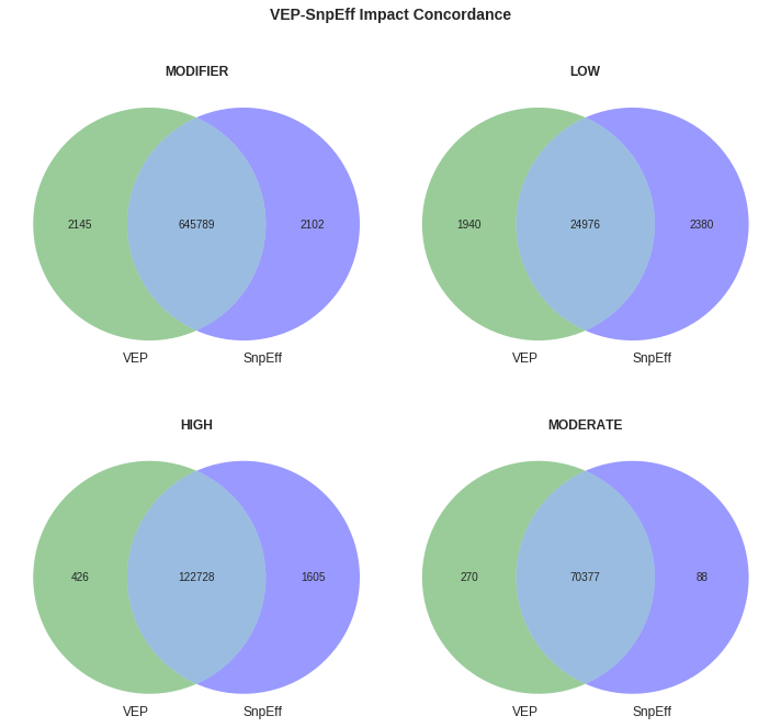
Concordance within various impact groupings is quite high across all buckets.
Looking at raw numbers we see the largest difference of produced effect terms among intergenic variants, which is unsurprising given that there is no firm definition between an intergenic and up or down stream variant. Moreover, since these variants are usually not included in clinical analysis, these mismatches are not worrisome.
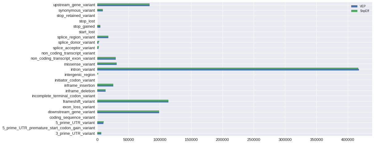
Absolute numbers of normalized effect terms produced by each algorithm are very similar.
The most problematic region for classification remains the area where exons are spliced together. For example, of the 2208 variants that VEP labels as splice_acceptor_variants, over 500 are labeled as something else by SnpEff. These labels range from stop_gained to conservative_inframe_deletion to splice_region. Thus, in this one set of effect mismatches, we find impacts from all categories.
Let’s dig into some of the mismatches and see if we can figure out what’s happening.
To simplify matters, I picked examples all on the canonical CFTR transcript ENST00000003084.
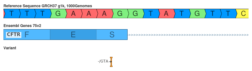
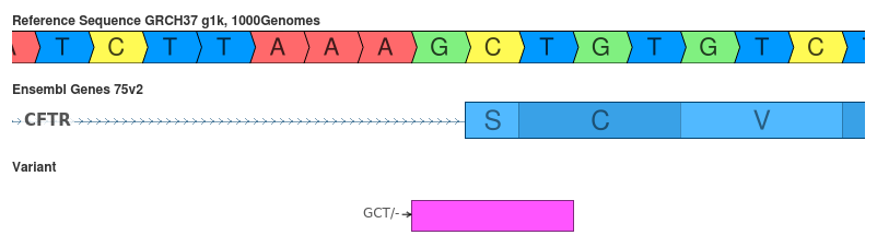
The effect of an GTA insertion is difficult to determine at this position.
If we examine the resultant coding sequence both interpretations are plausible. First, we can imagine that the inserted GT will produce the motif defining the splice site, thus moving the splice site 1 base 5’ of the the reference. Alternatively, the first two bases of the insertion with the preceding A will produce an ATG codon. This codon will push out the splice site 3 bases to the 3’ end of the transcript. This later interpretation implies the insertion of an additional Serine to the primary protein sequence, whereas the former (splice_donor_variant) interpretation implies a 1 base removal causing a frameshift that will propagate over the remaining sequence. My hunch would be to label this as a splice_donor_variant to prevent false negative results, but it is unclear what actually will occur during protein synthesis.
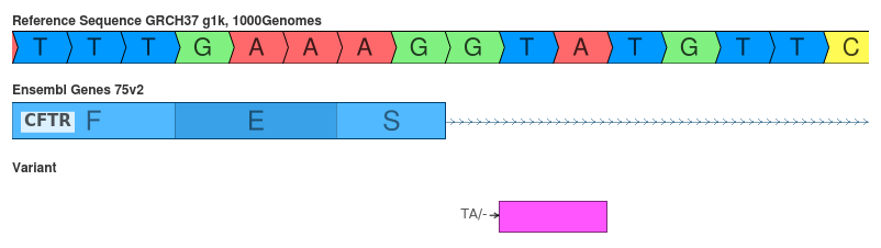
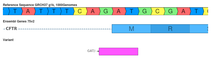
The interpretation of this variant can depend on the variant’s representation.
This variant is interesting because the interpretation depends on the variant’s representation. On its face, the deletion of the TA affects the position of the GT motif of the splice site. However, this variant is functionally equivalent to the deletion of the neighboring AT since the resultant sequence will retain the GT motif. This interpretation is reflected by the HGVS cDot notation produced. HGVS specifies that variants are to be shifted to their most 3’ position since this is how the DNA would be transcribed. In fact, SnpEff mentions that it specifically addresses this problem:
In order to report annotations that are consistent with HGVS notation, variants must be re-aligned according to each transcript’s strand (i.e. align the variant according to the transcript’s most 3-prime coordinate). Then annotations are calculated, thus the reported annotations will be consistent with HGVS notation.
This decision changes the impact of the variant from HIGH to LOW, thus likely removing it from consideration in downstream analysis.
SnpEff’s interpretation makes some deeper inferences about the variant to produce it’s less deleterious prediction.
VEP’s interpretation of this variant is straightforward since it appears that this variant disrupts the splice acceptor site. However, by 3’ shifting the variant SnpEff cleverly detected that the AG motif will still be intact. Thus the variant will change the Serine-Cysteine to an Arginine in the primary protein sequence.
Another disagreement caused by the decision to shift (or not) the variant to its 3’ representation.
This variant is another example of the inconsistency that can arise from the decision to 3’ shift the variant. VEP doesn’t do this shift prior to making its interpretation thus causing the disagreement.
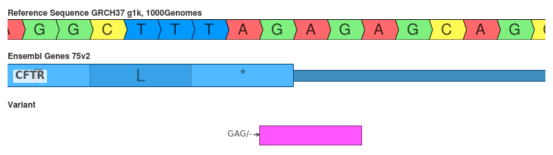
This variant shows how the space (DNA, RNA, AA) in which the variant is represented can influence the interpretation.
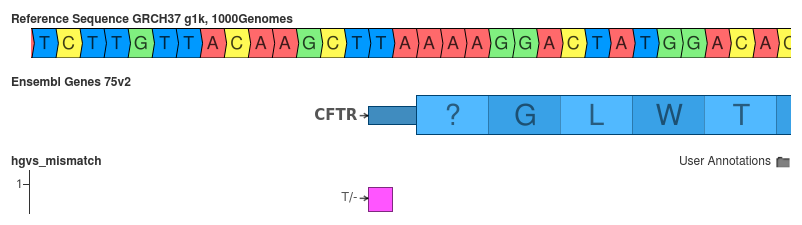
The interpretation of this variant is very tricky. Functionally, the deletion of the GAG changes the last codon for TAG to TAA. Both sequences are stop codons so they should function in a similar manner. However, since the triplet differs 3’ shifting in DNA (or RNA) space fails. Both algorithms seem to construct their HGVS notation from comparing the amino acid sequence and translating back to coding space. This is why both say that it is the second GAG repeat that is deleted in their HGVS construction. But overall, I think VEP gets this one right.
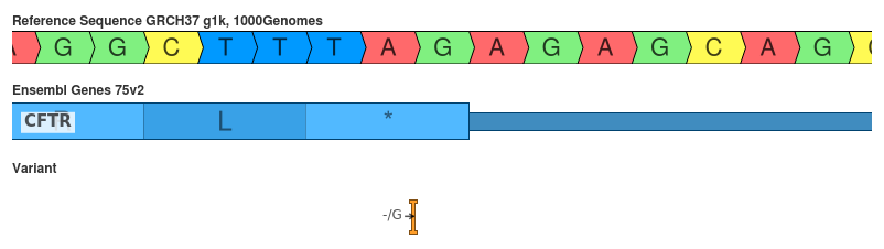
The insertion of a G should not change the final codon, but does change the 3’ UTR.
The duplication of the last G in the final codon should not change the primary sequence of the protein. However, it does change the 3’ UTR so SnpEff seems to have interpreted this correctly. Again this disagreement is due to VEP not 3’ shifting prior to interpretation.
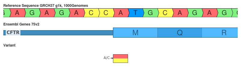
Alternate start codons are a source of legitimate disagreement.
This SNP changes the Methionine to Leucine. Although Met is the common initiation codon, Leu has been reported to serve as a alternate start codon. This research focused on the synthesis of peptides used in MHC molecules. Given the specific context of this behavior, I’d be wary of discounting this mutation as simply pseudo-synonymous. Perhaps the prediction of initiator_codon_variant is reasonable, but marking it as LOW impact might eliminate it from further analysis.
In addition to looking at effect and impact prediction, I also compared the HGVS coding sequence representations that each algorithm produces. I expected the concordance to closely match the effect concordance due to the fact that HGVS assumes that the description generator is aware of the relative location of transcript features (e.g. the variant is 1 base intronic thus implying a splice donor/acceptor effect).
Instead, I found only a 69% rate of agreement between generated HGVS notations. However, this value overstates the degree of mismatch since it doesn’t exclude variants where one algorithm doesn’t generate a HGVS identifier. Since many variants are intergenic, it’s unlikely that a cDot notation would (or should) be generated. Once the set of variants is limited to those for which both algorithms generate a identifier, the rate of concordance climbs to 88%.
Nonetheless, a 12% rate of disagreement is quite poor in an identification scheme which is designed to be unambiguous and objective. This rate of mismatch continues to support my position that these notations must be used cautiously and never as a unique identifier during data analysis workflows. Since clinical interpretations almost always include the HGVS identifier in reports, the clinician (and bioinformatic team) must be very diligent about checking the identifiers prior to releasing their findings.
From a cursory examination it appears that many variant representations don’t match due to the way each algorithm constructs transcripts. In fact, on the canonical transcript “ENST00000003084”, which is well characterized, we find no disagreements among variants which have an HGVS identifier produced by both SnpEff and VEP. To see how transcript representation causes differences, let’s look a one specific case.
The representation of the transcript can influence the generated HGVS identifier.
Is correct HGVS notation is what SnpEff yields: ENST00000468795:c.-2delT. Since it is two bases 5’ of the annotated start position of the transcript its position should be written as -2. Right? But, if you look at Ensembl’s notes abot this transcript, it states at the the “5’ UTR is incomplete”. Thus, if there isn’t a UTR, than VEP might be correct.
The reason I highlight this case is to show an assumption inherent in my analysis – that trascript representations are equivalent.
I am comparing variants projected into the entire transcript set provided by Ensembl. Many of the transcripts (including this one) are not well formed. By this I mean that their representation in genomic space is poor. For example, this transcript has a non-sensical start codon. Perhaps that is due to an error in the underlying RNA data from which this transcript is identified? Maybe the alignment algorithm couldn’t perfectly align it to the reference, and punting the start codon is the best it could do? Whatever the reason, we see the effects of poor transcript representation propagate into HGVS identifier production.
VEP assumes that the first base of the “UTR” is the first coding base, thus giving the identifier as ENST00000468795:c.1delT. Is this wrong? Yes if you believe the transcript in the preceeding figure is accurately represented. No, if you don’t think that the UTR is real. My preference would be that no HGVS identifier should be produced since the CDS start is not well defined.
Thus, even if you believe that the HGVS specification is perfectly clear, contains no ambiguities and always produces a unique identifier, the produced identifier still is premised upon how the transcript is represented. This need for well defined transcripts is why HGVS recommends using LRGs as accessions for coding DNA notations when possible.
This analysis didn’t even attempt to delve into the problems posed by the mismapping of transcripts to the reference sequence. However, the improvements in GRCh38 have been said to help decrease the prevalence of this problem.
I want to commend both of the developers of these algorithms on the accuracy they’ve been able to achieve. Having written an in-house version of this class of algorithm at Golden Helix, I know what a challenge it is. With the introduction of the ANN field and standardized sequence ontology, bioinformatics has taken a big step toward reproducibility and compatibility. Honestly, I don’t know if I would ever expect significantly more concordance in effect prediction. The last bit of “low hanging fruit” appears to be agreeing to 3’ shift variants prior to interpretation. Some small gains are likely to come from increasing the integrity of the input data by creating more accurate transcript maps and more consistent variant calls. The remaining differences are rooted in pushing the predictions to be more specific and nuanced.
The key takeaways of this analysis are:
And perhaps the most important thing to recognize is that the decisions made upstream in the bioinformatic pipeline will influence your results and the only way to compensate for these potential differences is to be aware of the pitfalls that are inherent in your analysis. That means having a good understanding of what the input data looks like, how your variant effect predictor functions, and how effects are treated downstream. If you have a good handle on these facets of your pipeline you shouldn’t find too many surprises in your data.